At a high level, bandit algorithms and supervised learning models can look surprisingly similar. In both cases, the goal is to look at a given context and predict the best class or “arm” to choose. For a recommendation system, this might mean predicting which product a user is most likely to click on.
But beneath this surface-level similarity lies a fundamental difference that dictates when and how you use each approach: the availability of feedback. This single distinction has massive implications for model training, adaptability, and real-world application.
The Core Difference: Partial vs. Full Feedback
Let’s break down the central conflict.
In a classic supervised learning problem, you operate with full feedback. Imagine you’re training a model to predict house prices. For every house in your training dataset, you have the full context (square footage, number of bedrooms, location) and the one true label (the final sale price). When training an image classifier, for each image of a cat, you know it’s a “cat” and not a “dog,” “bird,” or “car.” The ground truth is known for all possibilities.
Bandit algorithms, on the other hand, operate in a world of partial feedback. You only receive a label (called a “reward”) for the action you actually take.
Consider a news website testing 10 different headlines for an article. You show one headline to a user and observe if they click. You get the reward (a click or no-click) for that single headline, but you have no idea what would have happened if you had shown one of the other nine. This “what if” data is missing.
This forces a critical trade-off: exploration vs. exploitation.
- Exploitation: Sticking with the headline that has performed best so far.
- Exploration: Trying out other, less-proven headlines to see if one might be even better.
If you only exploit, you might get stuck with a locally optimal choice, never discovering a globally better one. Bandits are designed to manage this trade-off, often starting with more exploration and gradually shifting to exploitation as they learn.
Key Distinctions at a Glance
| Feature | Bandit Algorithms | Supervised Learning |
| Learning Style | Learns while acting (online); feedback is only for actions taken. | Learns from a fixed, fully labeled dataset (offline). |
| Feedback | Partial Feedback: Only for the chosen arm(s). | Full Feedback: Labels are known for all classes (or aggregated to be pseudo-full). |
| Adaptability | Always Learning: Continuously optimizes for the present and adapts to changing environments in real-time. | Stable & Predictable: Models are trained and validated offline. Less adaptive to live changes. |
| Exploration | Higher “Regret”: Must show some suboptimal options to users in order to explore and learn. Balances exploration and exploitation | No “Exploration Cost”: Doesn’t show suboptimal results to users. Can reinforce existing biases. Purely exploitation from offline learning. |
| Use Cases | Online ad selection, dynamic A/B testing, cold-start recommendations, dynamic pricing | Image classification, spam detection, core search ranking. |
| Model Complexity | Tends toward simpler models that can be updated instantly. | Can use extremely complex models (e.g., DNNs) trained over days or weeks. |
| Cold-Start | Excellent: A natural fit for discovering the value of new items or content. | Poor: Works well for behaviors and items seen during training, but struggles with newness. |
| Optimization | Optimizes for cumulative reward over time | Optimizes for error between prediction and ground truth |
When to Use Supervised Learning: The Full-Feedback Powerhouse
Supervised learning is the powerhouse behind most large-scale search and recommendation systems. You use it when you can build a complete, labeled dataset for offline training.
1. Training with Human-Generated Labels
- Scenario: A search engine employs human raters to judge the relevance of thousands of web pages for a given query (e.g., “Perfect,” “Good,” “Bad”).
- Why it Works: You have ground-truth labels for many possible results for a given query. The partial feedback problem doesn’t exist. This allows you to train a complex learning-to-rank model like LambdaMART to order results with high precision.
2. CTR Prediction with Aggregated Historical Logs
- Scenario: An e-commerce site has months of data showing which products users clicked on or purchased for popular queries like “blue sneakers.”
- Why it Works: For a popular query, you have data from thousands of users interacting with hundreds of products. By aggregating this log data, you can confidently estimate the click-through rate (CTR) or purchase probability for each product in that context. The partial feedback problem is effectively averaged away by the sheer volume of data.
When to Use Bandit Algorithms: The Online Optimizer
Bandits excel at making real-time decisions under uncertainty, especially when data is sparse or the environment is changing. They are used for online learning and optimization.
1. Recommending New or “Cold-Start” Items
- Scenario: A new article is published, or a new product is added to your store. Your offline supervised model has never seen it and gives it a low score by default.
- Why Bandits? A bandit can be instructed to “explore” this new item by showing it to a small fraction of users. If it gets a good response (clicks, purchases), the bandit will automatically show it more often, solving the cold-start problem in real-time. The New York Times famously uses bandits to test headlines for new articles.
2. Live A/B/n Testing and UI Choices
- Scenario: Should you show a user a “5% off” coupon or a “free shipping” banner? You can only show one and observe the result.
- Why Bandits? This is a classic partial feedback problem. A contextual bandit learns over time which promotion works best for which type of user, dynamically allocating traffic to the winning variant.
3. Fine-Tuning an Existing Ranking (Rank Exploration)
- Scenario: Your main supervised model provides a ranked list of 100 items. You’re confident about the top 3 but less sure about the order of items from 4-20.
- Why Bandits? You can use a bandit to slightly re-rank the items in the uncertain part of the list. It explores different orderings and learns which items perform better in those slots, gathering valuable data that can be fed back into your next offline training cycle.
Better Together: The Modern Hybrid System
In a sophisticated modern system, supervised learning and bandits are not mutually exclusive; they work together.
The supervised model does the heavy lifting offline, while the bandit handles the “last-mile” optimization online.
Supervised Model (Offline): “Based on all our historical data, these 100 products are the most relevant for this user. Here they are, ranked by predicted purchase probability.”Bandit Algorithm (Online): “Thanks. The main model is confident about the top 5, so I’ll show those. But for positions 6-10, I’ll explore by shuffling the items to see if we can discover something better. I’ll also mix in this brand-new product that the main model knows nothing about. I’ll see what the user clicks on and update my strategy for the next user instantly.”
This hybrid approach gives you the best of both worlds: the predictive power of a massive, offline-trained model and the adaptive, real-time learning of an online bandit algorithm.
Example: LinUCB vs Linear Regression
Imagine launching a website with 5 possible headlines. Each visitor arrives with a 5-feature context (e.g., device, location, referrer, time, past behavior). You must choose one headline to display and only observe the reward for that choice (e.g., click or dwell time). This is a classic contextual bandit problem: at each round, you see context-feature vectors for each arm (headline), pick one arm, and receive its reward. The goal is to maximize cumulative reward while learning which headline performs best for which user context.
LinUCB is a common contextual bandit algorithm for this setting. It assumes the expected reward is linear in the features of the user–headline pair and selects arms using an upper confidence bound (UCB) that trades off exploitation (predicted reward) and exploration (uncertainty).
How LinUCB works:
- Model: E[r | x] ≈ θᵀx, where x is the feature vector for a user–headline pair and θ is unknown.
- For each headline a with context x:
- Estimate θ via ridge regression from past data.
- Predicted reward: μ̂ = xᵀθ̂.
- Uncertainty: s = sqrt(xᵀA⁻¹x), where A is the design matrix.
- UCB score: p = μ̂ + α·s, with α controlling exploration.
- Choose the headline with the highest p, observe its reward, and update A and b (the sufficient statistics) so future estimates become more confident.
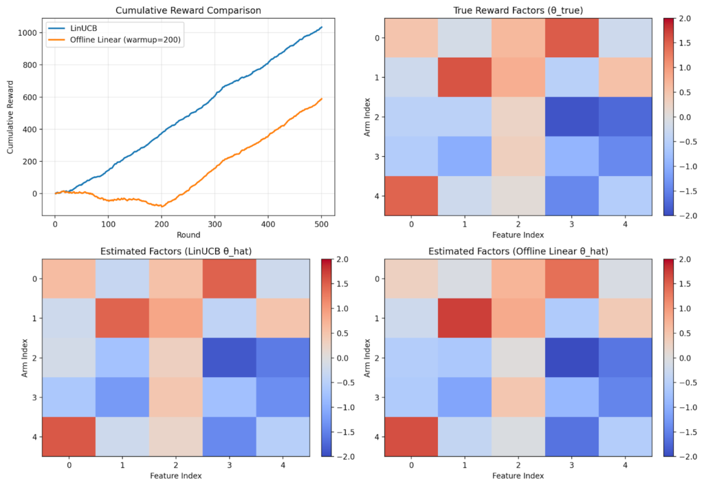
Below is a sample demo which performs LinUCB on the above problem with 5 features and 5 arms. Notice that UCB exploration reduces over time and reward stabilizes over time.
Formulation as Linear Regression
Alternatively, we could frame this as supervised learning. For the first K users, randomly select an arm and record the reward. This yields training data of the form (user features U, arm A, reward R), which we can use to fit a supervised linear model. The downside is that those initial K users may receive lower-quality results during data collection..
In this setting, linear regression models the expected reward as a linear function of the features describing a user–arm (headline) pair.
- Inputs: For each impression, build a feature vector x that encodes the user’s attributes (e.g., device, location) and the chosen headline (e.g., one-hot indicator or headline embeddings). Optionally include interaction terms between user and headline features.
- Target: The observed reward r (e.g., click = 1, no click = 0, or a continuous engagement metric).
The model:
- Assume E[r | x] ≈ θ^T x, where θ are coefficients to learn.
- Fit θ by minimizing squared error over collected data: sum_i (r_i − θ^T x_i)^2, typically with regularization (ridge/L2) to prevent overfitting and stabilize estimates.
The figure compares LinUCB with a supervised linear regression approach. With linear regression, the first ~200 impressions perform poorly because the system randomly explores to collect training data. In contrast, LinUCB balances exploration and exploitation from the start by using an uncertainty-aware bonus, yielding better early performance and a smoother user experience.
Design Considerations:
- Hybrid Approach: Once LinUCB has collected initial data through balanced exploration, this data can be used to train a more complex model offline for improved accuracy and better capturing of complex features.
- Feature engineering matters: Use normalized, bounded features; include interaction terms if plausible.
- Per-arm vs. Shared LinUCB: Use separate A_a, b_a per arm when arms differ or share little structure; use a single shared A, b across all arms when a common θ plausibly maps features to rewards—common in recommendation with shared feature representations. Shared setups leads to faster convergence on common features but the weight θ will be shared across all arms. This can lead to non-optimal solution where different weights for each arm is required. Read more in reference 1 and 2.
- LinUCB can capture stochastic nature of rewards. r ~ N(x,y)
- LinUCB assumes homoscedastic noise and a fixed uncertainty model, so it doesn’t naturally handle heteroscedasticity—situations where noise (or desired exploration) varies across variable range. For instance, if you have an upstream confidence score as a context feature and want more exploration when confidence is low and less when it’s high, vanilla LinUCB can’t learn that variability. As a simple workaround, use feature engineering to encode this behavior explicitly (e.g., add indicators like is_low_score = score < k and is_high_score = score > k), or consider heteroscedastic bandit methods (https://arxiv.org/pdf/1909.09146) that model context-dependent uncertainty directly.
- Standard LinUCB assumes stationary—the reward distribution is stable over time. For non-stationary settings (e.g., shifting user preferences or market conditions), use variants with decay or time-weighted updates to adapt the model to recent data.
- Linear assumption may be too simple in LinUCB; consider LinTS (linear Thompson sampling) or nonlinear methods (NeuralUCB) if non linearity is needed.
- Curse of Dimensionality: Adding more features into the model leads to more exploration and requires more samples to lead to convergence. This is required to get enough sample for each feature combinations. Dimensionality reduction and feature engineering is commonly used to reduce features for faster convergence.
Closing: Choosing the Right Tool for the Job
The choice between supervised learning and contextual bandits ultimately comes down to understanding your feedback structure and operational constraints. Supervised learning excels when you have abundant historical data, can afford offline training cycles, and need to leverage complex models for stable, well-understood prediction tasks. Contextual bandits shine when you must learn on-the-fly, face the cold-start problem, or operate in dynamic environments where the cost of exploration is acceptable for the gain of discovering better strategies.
As the LinUCB example illustrates, bandits don’t just match supervised learning’s eventual performance—they provide a fundamentally better user experience during the learning phase by intelligently balancing exploration and exploitation from the first interaction. Rather than subjecting early users to random experiments, bandits use principled uncertainty quantification to explore smartly while still delivering reasonable results.
In practice, the most powerful systems recognize that this isn’t an either-or decision. By combining the scalability and predictive power of offline supervised models with the adaptability and exploration capabilities of online bandits, you can build recommendation and decision systems that are both accurate and responsive—learning continuously from every interaction while maintaining the stability and performance users expect. The key is recognizing which problems require full feedback and offline optimization, and which demand the real-time learning and partial-feedback handling that only bandits can provide.
Code for Generating Images: LinUCB vs Supervised, LinUCB Animation