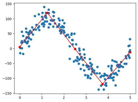
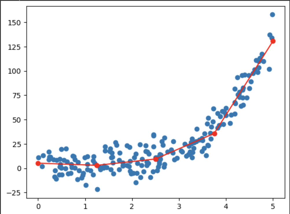
In this blog, I will train a simple piecewise linear curve on a dummy data using pytorch. But first, why piecewise linear curve? PWL curves are set of linear equation joined at common points. They allow you to mimic any non linear curve and their simplicity helps you explain the predictions. Moreover, they can be easily deployed and scaled. You can also add constraints like monotonicity in these curves.

So, Let’s get started.
PWL curves can be thought as similar to training a regression model, but instead of the output being function of single curve, it is output of multiple curves.
Bounded vs Unbounded: Linear curves are generally unbounded in nature as they can be directly applied to values outside of their training data. The same can be said about PWL curves as well. One can either set the values as min and max of the curve in training data or apply the first and last curve for out of bound inputs. For the purpose of this example, we will use min and max of the curve values for out of bound inputs. The estimation of range of input values are important for the finding appropriate points to create curve along
Input Range and Curve Points: The first step in training a PWL curve is to determine points between which the linear curves will be created. There are multiple heuristics that can be used here. One strategy could be to use different percentiles of input points across the range. This would ensure that each curve gets an equal number of points for training. Another strategy could be to simply take k equidistant points between min and max. For our example, we implement the latter strategy.
self.xranges = torch.linspace(start, end, ncurves + 1)PWL Representation and Training Parameters: A PWL Curve can be represented with a set of x points as shown above and a set of y points which represents the value of the curve at the x points. During inference, we identify which curve should be used based on the input and x points and generate prediction using that curve. Since, our x points are fixed, we train the set of y parameters at those x points.
$$ PWL_n = \{(x_1, y_1), (x_2, y_2), …, (x_n, y_n)\} $$
$$ \text{PWL}_n(x) = \text{Linear}(x, x_i, x_{i+1}, y_i, y_{i+1}) \quad \text{for } x_i < x <= x_{i+1} $$
$$ \text{Linear}(x, x_i, x_{i+1}, y_i, y_{i+1}) = \frac{y_{i+1}-y_i}{x_{i+1}-x{i}} (x-x_i) + y_i $$
class PWL(torch.nn.Module):
  def __init__(self, ncurves=3, rng=(0, 5)):
    super().__init__()
    start, end = rng
    self.xpoints = torch.linspace(start, end, ncurves + 1)
    self.weights  = torch.nn.Parameter(torch.randn(ncurves + 1,))

  def calculateLinear(self, x, start, end, ystart, yend):
    # y−y2=(y2−y1)(x2−x1)×(x−x2), equation of straight line
    y = (yend-ystart) / (end-start) * (x-start) + ystart
    return y

  def forward(self, x):
    # This could be optimized using binary search for large number of curves
    if x <= self.xpoints[0]:
      return self.weights[0]
    for i, (start, end) in enumerate(zip(self.xpoints[:-1], self.xpoints[1:])):
      if x > start and x <= end:
        return self.calculateLinear(x, start, end, self.weights[i], self.weights[i+1])
    if x > self.xpoints[-1]:
      return self.weights[-1]
  def forward(self, x):
    # This could be optimized using binary search for large number of curves
    if x <= self.xpoints[0]:
      return self.weights[0]
    for i, (start, end) in enumerate(zip(self.xpoints[:-1], self.xpoints[1:])):
      if x > start and x <= end:
        return self.calculateLinear(x, start, end, self.weights[i], self.weights[i+1])
    if x > self.xpoints[-1]:
      return self.weights[-1]
Training Strategy: We train the PWL curve similar to how we perform regression. We calculate the error between output and prediction and back propagate the loss to our input parameters.
def train(model, x, y):
  optimizer = torch.optim.SGD(model.parameters(), lr=0.1)
  for epoch in (pbar:=tqdm.tqdm(range(500))):

      # Forward pass
      y_pred = [model(i) for i in x]
      error = [(pred-act)**2 for pred, act in zip(y_pred, y)]

      # Loss Calculation
      loss = 0
      for e in error:
        loss = loss + e
      loss = loss / len(error)
      loss_scalar = loss.detach().numpy()
      pbar.set_description(f"Epoch: {epoch}, Loss: {loss_scalar:.2f}")

      # Backward pass
      loss.backward()

      # Update the parameters
      optimizer.step()

      # Clear the gradients
      optimizer.zero_grad()

  return loss_scalar
Sample Training and Curve:


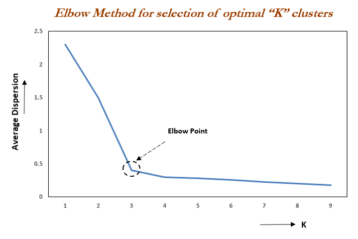
Finding Optimal Number of Curves Using Elbow Curve: Elbow curve is generated by calculating the optimum loss while increasing hyperparameter (number of curves). As the number of curves increases, the loss goes down. Because the model is now able to learn more complex characteristics from the data. A sudden drop in loss should be observed as model moves from underfitting to overfitting. After this, only incremental improvements can be observed. The number of curves after the this sudden drop is can be take as number of curves.

Elbow method is generally used for clustering to find number of cluster, but this can be generally applied to any learning algorithm which has a hyper parameter to increase the complexity of learning algorithm. Alternatives to this method can be found in related reads.
Advantage over Polynomial Regression?
- Less over fitting to number of data points: polynomial regression tends to overfit to locations where the number of samples are higher (because they contribute higher to losses)
- Simple to explain and understand the curve
Closing and Future Direction
PWL Curves are generally used to train GAM models (Generalized additive models) as these can be trained individually for multiple features. You can find the complete code along with working example in this colab. An important extension from this could be to learn the split points from data instead of using heuristics as above. Thanks for reading and keep learning!
PS: The current implementation in PyTorch is not efficient as it doesn’t accept the batch input. Leaving that as an exercise.
Related Reads:
- https://towardsdatascience.com/are-you-still-using-the-elbow-method-5d271b3063bd Are You Still Using the Elbow Method?
- https://arxiv.org/abs/2101.08393, Distilling Interpretable Models into Human-Readable Code
- https://github.com/google/pwlfit, PWLFit is a small library to fit data with a piecewise linear function.